Potential Model for Actinide Oxides (v1.0)
Many Bodied Actinide Oxide Potentials
We have developed a new potential model describing a range of actinide oxides which includes many-body effects to improve the description of their thermo-mechanical properties.
- Enquiries:
This work is published in: M.W.D. Cooper, M.J.D Rushton, R.W. Grimes, J. Phys. Condens. Matter 26 (2014) 105401.
We would be grateful if you could cite this paper if you make use, or derive, any work from the materials contained here.
This page provides a brief description of the model and gives examples of its ability to reproduce thermal expansion, elastic properties and specific heat for a wide range of actinide oxide systems:
- CeO2
- ThO2
- UO2
- NpO2
- PuO2
- AmO2
- CmO2
Importantly the oxygen-oxygen interactions are fixed across the actinide oxide series keeping open the ability to model mixed oxides. Currently this page hosts descriptions of the model suitable for the GULP and LAMMPS codes, we will be providing tabulation files for DL_POLY in the near future. Furthermore, we will be releasing the EAM tabulation python library used during the development of the model in the next few weeks. If you haven any questions please get in touch.
##Overview
Downloads
| File | Description |
|---|---|
| GULP_Example_UO2.zip | Example GULP UO2 energy minimisation. See below for more. |
| GULP_AmO2.lib | GULP AmO2 potential library file. |
| GULP_CeO2.lib | GULP CeO2 potential library file. |
| GULP_CmO2.lib | GULP CmO2 potential library file. |
| GULP_NpO2.lib | GULP NpO2 potential library file. |
| GULP_PuO2.lib | GULP PuO2 potential library file. |
| GULP_ThO2.lib | GULP ThO2 potential library file. |
| GULP_UO2.lib | GULP UO2 potential library file. |
| LAMMPS_example.zip | LAMMPS energy minimisation and equilibration run for UO2. Described in more detail below |
| LAMMPS_AmO2.fs | LAMMPS pair_style eam/fs potential tabulation for AmO2
|
| LAMMPS_CeO2.fs | LAMMPS pair_style eam/fs potential tabulation for CeO2
|
| LAMMPS_CmO2.fs | LAMMPS pair_style eam/fs potential tabulation for CmO2
|
| LAMMPS_NpO2.fs | LAMMPS pair_style eam/fs potential tabulation for NpO2
|
| LAMMPS_PuO2.fs | LAMMPS pair_style eam/fs potential tabulation for PuO2
|
| LAMMPS_ThO2.fs | LAMMPS pair_style eam/fs potential tabulation for ThO2
|
| LAMMPS_UO2.fs | LAMMPS pair_style eam/fs potential tabulation for UO2
|
##Using the Model in LAMMPS [id_lammps_model]
Example
In order to show how the potential model can be used in LAMMPS a working example has been provided. The LAMMPS_example.zip provides an example where a 4×4×4 UO2 super-cell is energy minimised then equilibrated under NPT conditions at a temperature of 300K for 50ps. This should give a good idea of how the other LAMMPS potential tabulations can be used.
Running the Example
- Unzip the LAMMPS_example.zip archive.
- In your terminal enter the example directory.
- Run LAMMPS:
lammps -in EAM_equil.lmpin -log EAM_equil.lmpout
Details
Both the EAM and pairwise interactions of the actinide oxide potential
described below are tabulated for use in LAMMPS
using the eam/fs pair_style, as described in the LAMMPS
manual. The pair_coeff
command is used to assign the elements within tabulated EAM file to
LAMMPS' species IDs. The following example shows how the LAMMPS_UO2.fs
table file is used in LAMMPS.
  pair_style hybrid/overlay coul/long ${SR_CUTOFF} eam/fs
  pair_coeff   *    *    coul/long
  pair_coeff   *    *    eam/fs embed_UO2.fs O U
Notes:
-
Oxygen is assumed to have ID = 1 and uranium ID = 2
-
NB: if the IDs were reversed, such that U = 1 and O = 2,
then then the species would be reversed in the
pair_coeffcommand as follows:pair_coeff * * eam/fs embed_UO2.fs U O
-
NB: if the IDs were reversed, such that U = 1 and O = 2,
then then the species would be reversed in the
-
pair_style hybrid/overlayis used to combinecoul/longwith the EAM model (eam/fs), this tells LAMMPS to calculate the electrostatic interactions between ions (NB: akspace_stylemust also be defined). -
Ion charges of 2.2208 for uranium and -1.1104 for oxygen should be specified. This can be performed either in a LAMMPS file read in using
read_dataor using theset chargedirective. The variable
${SR_CUTOFF}is used to define the cut-off parameter forcoul/long.
Using the Model in GULP
GULP library files are provided for each actinide oxide. These can be downloaded using the links in the downloads table.
Example:
An example showing how to energy minimise a single fluorite UO2
unit-cell using the GULP_UO2.lib file is provided in the
GULP_Example_UO2.zip.
Running the Example
- Unzip GULP_Example_UO2.zip.
- From the terminal enter the example directory
- Run the provided GULP file:
gulp < GULP_UO2_fluorite_example.gin
Note: The other GULP libraries provided within the
downloads table can be used with the
GULP_UO2_fluorite_example.gin by changing the library directive to
refer to another model file.
Details
In GULP the actinide oxide potentials are defined using the species, buck, morse, manybody, eam_functional and eam_density keywords without the need for tabulation. Ionic charges for the description of Coulombic interactions are defined using the species keyword.
  species 2
  U      core    2.220800
  O      core   -1.110400
Short range Buckingham and Morse parameters are defined using the buck and morse keywords respectively.
  buck
  O     core U     core  448.778865087 0.387757677453 0.0  0.00 11.00
  O     core O     core  830.283447557 0.352856254215 3.88437209048  0.00 11.00
  U     core U     core  18600.0 0.27468 0.0  0.00 11.00

  morse
  O     core U     core  0.6607973133 2.05815247834 2.38051231271  0.000 11.000
The short range and long range cut-offs for the Embedded Atom Method (EAM) are defined using the manybody keyword.
  manybody
  O     core U     core  1.500 11.000
  U     core U     core  1.500 11.000
  O     core O     core  1.500 11.000
The square root form of the embedding function and associated \(G_\alpha\) parameters are defined using the eam_functional keyword.
  eam_functional square_root
  U     core         1.8061282781
  O     core         0.690017059438
The \(\sigma_\beta(r_{ij})\) functions and associated
\(n_\beta\) parameters are defined using the eam_density keyword.
  eam_density power  8
  U     core         3450.99492623
  O     core         106.855913747
##Model Description and Parameters [id_model_description]
Our approach used the embedded atom method to introduce many-body effects to the more conventional Buckingham + Morse pairwise description. This approach is advantageous as it allows the inclusion of many-body interactions in MD simulations without the tricky massless entities required by the shell model.
The actinide oxide potential set has two distinct components: pairwise and many-body. The energy, \(E_i\), of atom \(i\) with respect to all other atoms can be written as follows:
\[
E_{\textit{i}} =
\color{orange} \frac{1}{2}\sum_\textit{j}\phi_{\alpha\beta}(r_{ij})
\color{magenta} -G_\alpha \sqrt{\sum_\textit{j}\sigma_{\beta}(r_{\textit{ij}})}
\]
Pairwise Component
The first, pairwise term describes short range cation-oxygen pair interactions. This uses the conventional Buckingham-Morse potential with long range Coulombic interactions also included:
\[ \definecolor{buck}{RGB}{255,0,0} \definecolor{coulomb}{RGB}{0,0,255} \definecolor{morse}{RGB}{0,128,0} \phi_{\alpha\beta}(r_{\textit{ij}}) =
\color{coulomb} \frac{q_{\alpha}q_{\beta}}{4\pi \epsilon_0 r_{\textit{ij}}} \color{black} +
\color{buck} A_{\alpha\beta}\exp \left(\frac{-r_{\textit{ij}}}{\rho_{\alpha\beta}}\right)-\frac{C_{\alpha\beta}}{r_{\textit{ij}}6} \color{black} +
\color{morse} D_{\alpha\beta}[\exp(-2\gamma_{\alpha\beta}(r_{\textit{ij}}-r_0))-2\exp(-\gamma_{\alpha\beta}(r_{\textit{ij}}-r_0))] \]
For Coulombic interactions the charges of the ions are non-formal such that \(q_\alpha=Z^{eff}_\alpha |e| \), however, they are proportional to their formal charges ensuring the system is charge neutral (for tetravalent cations \(Z^{eff}_\alpha\) = 2.2208 and for oxygen \(Z^{eff}_\alpha\) = -1.1104 ). \(A_{\alpha\beta}\), \(\rho_{\alpha\beta}\), \(C_{\alpha\beta}\), \(D_{\alpha\beta}\), \(\gamma_{\alpha\beta}\) and \(r_0\) are empirical parameters that describe the Buckingham and Morse potentials. For cation-cation and oxygen-oxygen interactions the covalent Morse term is not required (i.e. D=0). The pairwise parameters are now summarised:
| Interaction | \(\phi_B (r_{ij})\) | \(\phi_M (r_{ij})\) | ||||
|---|---|---|---|---|---|---|
| \(\alpha - \beta\) | \(A_{\alpha\beta}\) / eV | \(\rho_{\alpha\beta}\) / Å | \(D_{\alpha\beta}\) / eV | \(\gamma_{\alpha\beta}\) / Å–1 | \(r_0\) / Å | |
| Ce-Ce | 18600 | 0.2664 | 0.0 | - | - | - |
| Th-Th | 18600 | 0.2884 | 0.0 | - | - | - |
| U-U | 18600 | 0.2747 | 0.0 | - | - | - |
| Np-Np | 18600 | 0.2692 | 0.0 | - | - | - |
| Pu-Pu | 18600 | 0.2637 | 0.0 | - | - | - |
| Am-Am | 18600 | 0.2609 | 0.0 | - | - | - |
| Cm-Cm | 18600 | 0.2609 | 0.0 | - | - | - |
| Ce-O | 351.341 | 0.3805 | 0.0 | 0.7193 | 1.869 | 2.356 |
| Th-O | 315.544 | 0.3959 | 0.0 | 0.6261 | 1.860 | 2.498 |
| U-O | 448.779 | 0.3878 | 0.0 | 0.6608 | 2.058 | 2.381 |
| Np-O | 360.436 | 0.3830 | 0.0 | 0.7638 | 1.840 | 2.368 |
| Pu-O | 377.395 | 0.3793 | 0.0 | 0.7019 | 1.980 | 2.346 |
| Am-O | 364.546 | 0.3774 | 0.0 | 0.7467 | 1.955 | 2.325 |
| Cm-O | 356.083 | 0.3775 | 0.0 | 0.7613 | 2.081 | 2.311 |
| O-O | 830.283 | 0.3529 | 3.8843 | - | - | - |
Embedded Atom Component
The second term uses the Embedded Atom Method to introduce a subtle many-body perturbation to the conventional pairwise description. This many-body dependency is achieved by summing a set of pairwise functions, \(\mathrm{\sigma_\beta(r_{ij})}\), between atom \(i\) and its surrounding atoms. \(\mathrm{\sigma_\beta(r_{ij})}\) is proportional to the 8th power of the inter-ionic separation with \(n_\beta\) being the constant of proportionality and is defined by the species of the surrounding atom \(j\):
\[\sigma_{\beta}(r_{\textit{ij}}) =\frac{n_{\beta}}{r_{\textit{ij}}^8}\]
\(\mathrm{\Sigma\sigma_\beta(r_{ij})}\) is then passed through a non-linear embedding function. The embedding function used means that the many-body energy perturbation is proportional to the square root of \(\mathrm{\Sigma\sigma_\beta(r_{ij})}\) with \(G_\alpha\) being the constant of proportionality and is defined by the species of atom \(i\). The EAM parameters are given in the following table:
| Species | \(G_\alpha\) / eVÅ1.5 | \(n_\beta\) / Å5 |
|---|---|---|
| Ce | 0.308 | 1556.803 |
| Th | 1.185 | 1742.622 |
| U | 1.806 | 3450.995 |
| Np | 0.343 | 1796.945 |
| Pu | 1.231 | 1456.773 |
| Am | 0.333 | 1631.091 |
| Cm | 0.494 | 1503.704 |
| O | 0.690 | 106.856 |
##Comparison with Experimental Data [id_model_validation]
The potential was successfully fitted for all actinide oxides to experimental data of thermal expansion via MD and elastic constants via static calculations. The agreement obtained between model predictions and experimental data is now given.
###Thermal Expansion: [id_graph_thermal_expansion]
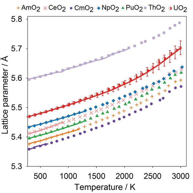
Comparison of experimental data (solid lines) with the data points from MD simulations obtained using the potential model for CeO2, ThO2, UO2, NpO2, PuO2, AmO2 and CmO2.
###Bulk Modulus: [id_graph_bulk_modulus]
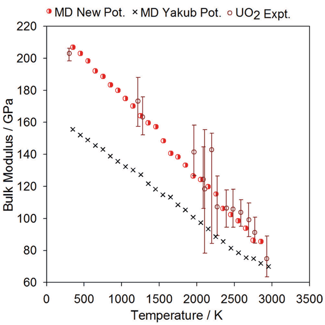
Comparison of experimental data for UO2 bulk modulus (open circles) with the data points from MD simulations (red half-circles) using the new potential.
###Specific Heat Capacity: [id_graph_specific_heat_capacity]
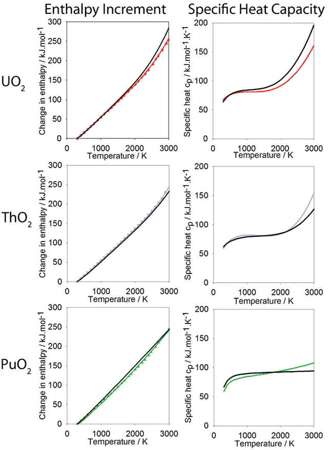
Change in enthalpy relative to 300K as a function of temperature calculated using the new potential. Polynomials have been fitted to the data for PuO2 ThO2 and UO2, shown in green, purple and red respectively. The polynomial form is based on that used for the experimental data, also shown in black. The derivative of the enthalpy gives the specific heat and is shown alongside the enthalpy data.