Potential Model for Actinide Oxides and their Solid Solutions
We have developed a new potential model describing a range of actinide oxides which includes many-body effects to improve the description of their thermophysical properties. The model has been developed to describe the following oxides and as of v1.1 of the model, their solid solutions: CeO2, ThO2, UO2, NpO2, PuO2, AmO2 and CmO2.
-
Enquiries:
- M.W.D Cooper, cooper_m@lanl.gov
- M.J.D. Rushton, m.rushton@imperial.ac.uk
Version History
| Versions | Description | Relevant Papers |
|---|---|---|
| v1.2 - 10/03/2015 | Modifications made to PuO2 parameters enabling the potential to reproduce the melting point. Updated tabulation files are provided | [1],[2],[3] |
| v1.12 - 21/01/2015 | Increased precision for parameters reported in tables and introduction of tabulation scripts to allow DL_POLY tabulation and modification of the model | [1],[2] |
| v1.11 - 10/11/2014 | Explanation of error function for short range cut-off on EAM | [1],[2] |
| v1.1 - 08/10/2014 | Model extended to allow simulation of mixed oxide (MOX) systems | [1],[2] |
| v1.0 - 09/01/2014 | Initial potential model as published in J. Phys. Condens. Matter | [1] |
- The model was originally published in:
- The extension of the model to mixed oxide solid solutions was published in:
- The modification of PuO2 parameters enabling the potential to reproduce the melting point:
We would be grateful if you could cite these papers if you make use, or derive, any work from the materials contained here.
This page hosts descriptions of the model suitable for the GULP and LAMMPS codes.
Overview
- Downloads
- Model Description and Parameters
- Pairwise Component
- Embedded Atom Component
- Mixed Cation-Cation Interactions
- Model Validation
- Properties of Single Actinide Oxide Systems
- Mixed Oxide System (U,Th)O2
- Using the Model in Common Simulation Codes
- Using the Model in LAMMPS
- Using the Model in GULP
Downloads_v1.2
| Version 1.2 Files | Description |
|---|---|
| GULP_MO2.lib | Gulp .lib containing potential parameters for all actinide oxides. |
| CeThUNpPuAmCmO.eam.alloy | LAMMPS tabulation for all actinide oxides for use with pair_style eam/alloy |
| GULP_Example_UO2.zip | Example GULP minimisation for UO2 |
| GULP_UThO2_example.zip | Example Mixed Oxide GULP minimisation |
| LAMMPS_example.zip | Example LAMMPS equilibration |
| LAMMPS_UThO2_example.zip | Example LAMMPS equilibration U, Th mixed oxide |
Note for DL_POLY Users: We are unable to provide a single TABLE file that supports all the actinide oxides and their solid solutions, however custom TABLE files can be generated for a particular DL_POLY simulation using the scripts provided here.
Model Description and Parameters
Our approach used the embedded atom method to introduce many-body effects to the more conventional Buckingham + Morse pairwise description. This approach is advantageous as it allows the inclusion of many-body interactions in MD simulations without the tricky massless entities required by the shell model.
The actinide oxide potential set has two distinct components: pairwise and many-body. The energy, \(E_i\), of atom \(i\) with respect to all other atoms can be written as follows:
\[
E_{\textit{i}} =
\color{orange} \frac{1}{2}\sum_\textit{j}\phi_{\alpha\beta}(r_{ij})
\color{magenta} -G_\alpha \sqrt{\sum_\textit{j}\sigma_{\beta}(r_{\textit{ij}})}
\]
Pairwise Component
The first, pairwise term describes short range cation-oxygen pair interactions. This uses the conventional Buckingham-Morse potential with long range Coulombic interactions also included:
\[ \definecolor{buck}{RGB}{255,0,0} \definecolor{coulomb}{RGB}{0,0,255} \definecolor{morse}{RGB}{0,128,0} \phi_{\alpha\beta}(r_{\textit{ij}}) =
\color{coulomb} \frac{q_{\alpha}q_{\beta}}{4\pi \epsilon_0 r_{\textit{ij}}} \color{black} +
\color{buck} A_{\alpha\beta}\exp \left(\frac{-r_{\textit{ij}}}{\rho_{\alpha\beta}}\right)-\frac{C_{\alpha\beta}}{r_{\textit{ij}}6} \color{black} +
\color{morse} D_{\alpha\beta}[\exp(-2\gamma_{\alpha\beta}(r_{\textit{ij}}-r_0))-2\exp(-\gamma_{\alpha\beta}(r_{\textit{ij}}-r_0))] \]
For Coulombic interactions the charges of the ions are non-formal such that \(q_\alpha=Z^{eff}_\alpha |e| \), however, they are proportional to their formal charges ensuring the system is charge neutral (for tetravalent cations \(Z^{eff}_\alpha\) = 2.2208 and for oxygen \(Z^{eff}_\alpha\) = -1.1104 ). \(A_{\alpha\beta}\), \(\rho_{\alpha\beta}\), \(C_{\alpha\beta}\), \(D_{\alpha\beta}\), \(\gamma_{\alpha\beta}\) and \(r_0\) are empirical parameters that describe the Buckingham and Morse potentials. For cation-cation and oxygen-oxygen interactions the covalent Morse term is not required (i.e. D=0). The pairwise parameters are now summarised:
NOTE: Modified PuO2 parameters are shown in bold.
| Interaction | \(\phi_B (r_{ij})\) | \(\phi_M (r_{ij})\) | ||||
|---|---|---|---|---|---|---|
| \(\alpha - \beta\) | \(A_{\alpha\beta}\) / eV | \(\rho_{\alpha\beta}\) / Å | \(C_{\alpha\beta}\) / eVÅ^6 | \(D_{\alpha\beta}\) / eV | \(\gamma_{\alpha\beta}\) / Å–1 | \(r_0\) / Å |
| Ce-Ce | 18600 | 0.2664 | 0.0 | - | - | - |
| Th-Th | 18600 | 0.2884 | 0.0 | - | - | - |
| U-U | 18600 | 0.2747 | 0.0 | - | - | - |
| Np-Np | 18600 | 0.2692 | 0.0 | - | - | - |
| Pu-Pu | 18600 | 0.2637 | 0.0 | - | - | - |
| Am-Am | 18600 | 0.2609 | 0.0 | - | - | - |
| Cm-Cm | 18600 | 0.2609 | 0.0 | - | - | - |
| Ce-O | 351.341 | 0.380517 | 0.0 | 0.71925 | 1.86875 | 2.35604 |
| Th-O | 315.544 | 0.395903 | 0.0 | 0.62614 | 1.85960 | 2.49788 |
| U-O | 448.779 | 0.387758 | 0.0 | 0.66080 | 2.05815 | 2.38051 |
| Np-O | 360.436 | 0.383047 | 0.0 | 0.76382 | 1.84020 | 2.36838 |
| Pu-O | 527.516 | 0.379344 | 0.0 | 0.70185 | 1.98008 | 2.34591 |
| Am-O | 364.546 | 0.377388 | 0.0 | 0.74668 | 1.95534 | 2.32486 |
| Cm-O | 356.083 | 0.377488 | 0.0 | 0.76128 | 2.08061 | 2.31107 |
| O-O | 830.283 | 0.352856 | 3.884372 | - | - | - |
Embedded Atom Component
The second term uses the Embedded Atom Method to introduce a subtle many-body perturbation to the conventional pairwise description. This many-body dependency is achieved by summing a set of pairwise functions, \(\mathrm{\sigma_\beta(r_{ij})}\), between atom \(i\) and its surrounding atoms. \(\mathrm{\sigma_\beta(r_{ij})}\) is proportional to the 8th power of the inter-ionic separation with \(n_\beta\) being the constant of proportionality and is defined by the species of the surrounding atom \(j\):
\[\sigma_{\beta}(r_{\textit{ij}}) =\left( \frac{n_{\beta}}{r_{\textit{ij}}^8} \right)\frac{1}{2}\left(1+\mathrm{erf}\left(20(r-1.5)\right) \right)\]
\(\mathrm{\Sigma\sigma_\beta(r_{ij})}\) is then passed through a non-linear embedding function. The embedding function used means that the many-body energy perturbation is proportional to the square root of \(\mathrm{\Sigma\sigma_\beta(r_{ij})}\) with \(G_\alpha\) being the constant of proportionality (see equation at top) and is defined by the species of atom \(i\). Due to the unrealistic energies that arise from the EAM at short distances an error function is applied at 1.5 Å that reduces the EAM contribution gradually. This ensures that there is no discontinuity near the bottom of the potential well that would arise from an abrupt cut off.
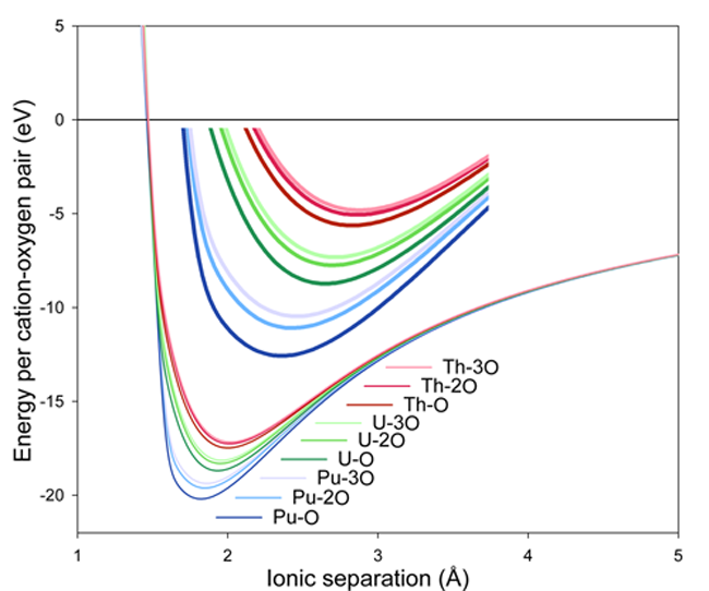
Using the EAM and pairwise parameters, the figure below shows the interaction energy as a function of interionic separation for Pu-O, Th-O and U-O interactions where the actinide is coordinated by one, two or three oxygen anions (O-O interactions are omitted). This plot reaffirms both the many-body nature of the potential and that the error function works well as a means of tapering the EAM at short distances.
NOTE: Modified PuO2 parameters are shown in bold.
| Species | \(G_\alpha\) / eVÅ1.5 | \(n_\beta\) / Å5 |
|---|---|---|
| Ce | 0.308 | 1556.803 |
| Th | 1.185 | 1742.622 |
| U | 1.806 | 3450.995 |
| Np | 0.343 | 1796.945 |
| Pu | 2.168 | 3980.058 |
| Am | 0.333 | 1631.091 |
| Cm | 0.494 | 1503.704 |
| O | 0.690 | 106.856 |
Mixed Cation-Cation Interactions
Although the O-O interactions have been kept consistent across the actinide oxide systems, it is still necessary to develop pair potentials that describe the interaction between two dissimilar cations (e.g. a U-Th potential). Similarly to the cation-cation interactions defined previously, the Buckingham A term is fixed at 18600 eV for all pairs of cations, whilst C parameters are set to zero. However, the mixed cation \(\rho_{\alpha\beta}\) parameters are defined in terms of the self cation-cation \(\rho_{\alpha\alpha}\) and \(\rho_{\beta\beta}\) terms using the following relationship:
\[\rho_{\alpha\beta}=(\rho_{\alpha\alpha}\rho_{\beta\beta})^{\frac{1}{2}}\]
| \(\rho_{\alpha\beta}\) | Ce | Th | U | Np | Pu | Am | Cm |
|---|---|---|---|---|---|---|---|
| Ce | 0.2664 | 0.2772 | 0.2705 | 0.2678 | 0.2651 | 0.2637 | 0.2637 |
| Th | - | 0.2884 | 0.2815 | 0.2786 | 0.2758 | 0.2743 | 0.2742 |
| U | - | - | 0.2747 | 0.2719 | 0.2691 | 0.2677 | 0.2677 |
| Np | - | - | - | 0.2692 | 0.2664 | 0.2650 | 0.2650 |
| Pu | - | - | - | - | 0.2637 | 0.2623 | 0.2623 |
| Am | - | - | - | - | - | 0.2609 | 0.2609 |
| Cm | - | - | - | - | - | - | 0.2609 |
Model Validation
The following section compares the model’s predictions with experimental data.
Properties of Single Actinide Oxide Systems
The potential was successfully fitted for all actinide oxides to experimental data of thermal expansion via MD and elastic constants via static calculations. The agreement obtained between model predictions and experimental data is now given.
Thermal Expansion:
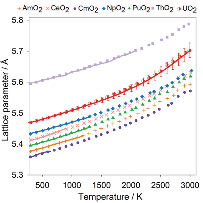
Comparison of experimental data (solid lines) with the data points from MD simulations obtained using the potential model for CeO2, ThO2, UO2, NpO2, PuO2, AmO2 and CmO2.
Bulk Modulus:
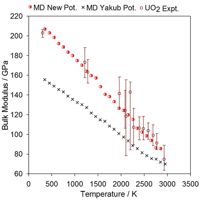
Comparison of experimental data for UO2 bulk modulus (open circles) with the data points from MD simulations (red half-circles) using the new potential.
Specific Heat Capacity:
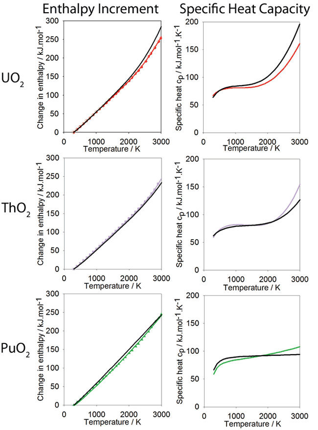
Change in enthalpy relative to 300K as a function of temperature calculated using the new potential. Polynomials have been fitted to the data for PuO2 ThO2 and UO2, shown in green, purple and red respectively. The polynomial form is based on that used for the experimental data, also shown in black. The derivative of the enthalpy gives the specific heat and is shown alongside the enthalpy data.
Mixed Oxide System (U,Th)O2
The results of simulations on the (U,Th)O2 system are given here to demonstrate the predictive ability of this model.
Thermal Expansion:
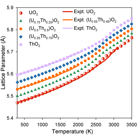
The lattice parameter as function of composition observes Vegard’s Law below 2000 K. Above this temperature, however, there is a ‘bump’ in lattice parameter associated with oxygen disorder.
Specific Heat Capacity:
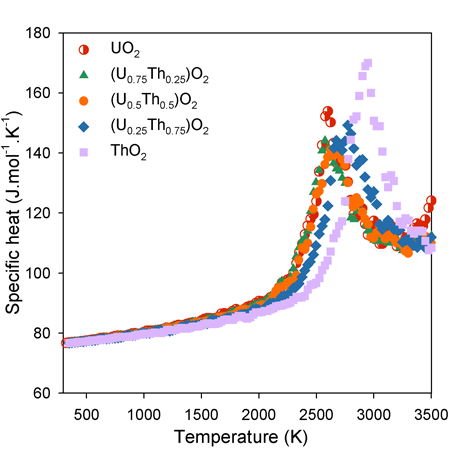
The increase in specific heat capacity as function of temperature is approximately linear below 2000 K. Above this temperature, however, there is a ‘bump’ in specific heat capacity associated with the enthalpy required to generate high temperature oxygen disorder.
Oxygen Diffusivity:
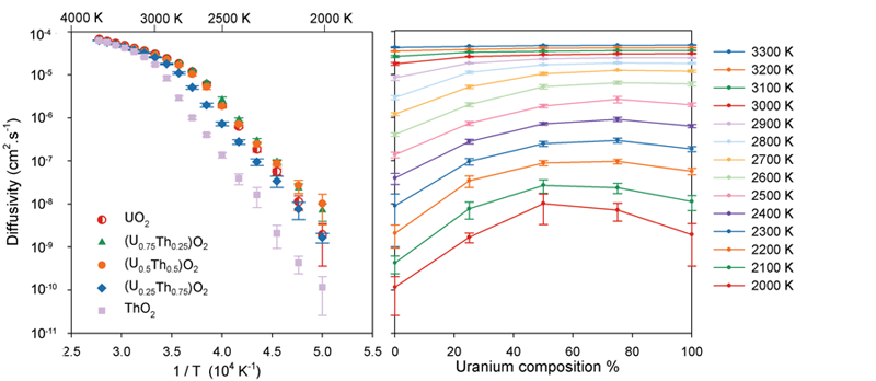
The change in gradient of the diffusivity as a function of temperature (left) indicates a change in the oxygen diffusion mechanism as the system undergoes the super-ionic transition. At low temperatures it is apparent that the solid solutions exhibit enhanced oxygen diffusivity relative to the end member systems.
Oxygen Defect Energies:
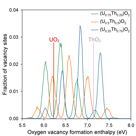
Unlike the end members, the solid solution oxygen sites that have a wide range of possible coordination environments due to the random distribution of U and Th on the cation sub-lattice. The peaks in vacancy formation enthalpy are associated with the 5 possible first nearest neighbour coordination environments of the oxygen sites - i.e. from lowest to highest enthalpy they are surrounded by 4, 3, 2, 1, and 0 uranium cations (or 0, 1, 2, 3 and 4 thorium cations).
All of the solid solutions contain a significant proportion of defect enthalpies that are lower in energy that for pure UO2. This contributes to the enhanced oxygen diffusivity.
Using the Model in Common Simulation Codes
Using the Model in LAMMPS
The following examples show how to use the relevant files within the Downloads table with the LAMMPS code.
Single Oxide Example
The LAMMPS_example.zip contains an example equilibration for a UO2 super-cell with the fluorite structure. See below for a thorough description of how the model is specified to LAMMPS.
To run the example, unzip the archive, enter its directory and type:
lammps -in EAM_equil.lmpin -log EAM_equil.lmpout
Mixed Oxide Example
In order to show how the MOX potential model can be used in LAMMPS a working example has been provided. LAMMPS_UThO2_example.zip provides an example where a 5×5×5 (U0.5,Th0.5)O2 supercell is energy minimised then equilibrated under NPT conditions at 300K for 50ps. This should give a good idea of how other mixed oxide systems can be simulated by modifying the .lmpstruct file.
Running the Example
- Unzip the LAMMPS_UThO2_example.zip archive.
- In your terminal enter the example directory.
- Run LAMMPS:
lammps -in EAM_NPT.lmpin -log EAM_NPT.lmpout
Details
Both the EAM and pairwise interactions of the actinide oxide potential described below are tabulated for use in LAMMPS using the eam/alloy pair_style, as described in the LAMMPS manual. The pair_coeff command is used to assign the elements within a tabulated EAM file to LAMMPS species IDs. The following example shows how the CeThUNpPuAmCmO.eam.alloy table file is used in LAMMPS.
  pair_style hybrid/overlay coul/long ${SR_CUTOFF} eam/alloy
  pair_coeff   *    *    coul/long
  pair_coeff   *    *    eam/alloy  CeThUNpPuAmCmO.eam.alloy  O Ce Th U Np Pu Am Cm
Notes:
- It is important to make sure the order in which the species appear in the
pair_coeffcommand is consistent with the IDs assigned in the.lmpstructfile. -
pair_style hybrid/overlayis used to combinecoul/longwith the EAM model (eam/alloy), this tells LAMMPS to calculate the electrostatic interactions between ions (NB: akspace_stylemust also be defined). - Ion charges of 2.2208 for uranium and -1.1104 for oxygen should be
specified. This can be performed either in a LAMMPS file read in
using
read_dataor using theset chargedirective. The latter approach is used in our example. - The variable
${SR_CUTOFF}is used to define the cut-off parameter forcoul/long.
Using the Model in GULP
The following examples demonstrate how to use the files provided in the Downloads table to perform simulations in the GULP code.
A single GULP library files is provided for all the actinide oxides and their solid solution. This can be downloaded using the link in the downloads table.
Single Oxide Example
An example showing how to energy minimise a single fluorite UO2 unit-cell can be found in GULP_Example_UO2.zip.
Running the Example
- Unzip GULP_Example_UO2.zip.
- From the terminal enter the example directory
- Run the provided GULP file:
gulp < GULP_UO2_fluorite_example.gin
Mixed Oxide Example:
An example showing how to energy minimise a single fluorite UO2
unit-cell with a Th cation substituted at one of the uranium sites using the GULP_MO2.lib file is provided in the
GULP_UThO2_example.zip.
Running the Example
- Unzip GULP_UThO2_example.zip.
- From the terminal enter the example directory
- Run the provided GULP file:
gulp < GULP_Th_in_UO2_example.gin
Note: The other actinide oxide systems can be studied by changing the structure inGULP_Th_in_UO2_example.gin without changing the library directive.